Chapter 3
Rationale for IID-based Panning
The audio engineer has several choices of localization cues when designing a pan pot. The type of playback system severely constrains how well these different cues will operate. Panning algorithms based on binaural, HRTF measurements are typically limited to headphone reproduction, ideally with head tracking devices. When these methods are used with loudspeakers in a room, two things degrade performance. (1) The right ear hears the signal meant for the left ear (and vice-versa), and (2) room reverberations give contradictory cues to localization. All HRTF methods are affected by the "goodness" of the original measurements; listeners may or may not localize well with someone else’s pair of HRTFs. Even if the listener’s HRTFs match the measured ones to a great extent, the effect still will be somewhat unnatural because the signal will pass through two HRTFs -- one more than normal.
Traditional theories of stereo are based on an open-air model of the head, one in which no head shadowing occurs for the contralateral ear. Cooper and Bauck [22] [23] discovered problems with shadowless stereo theory and developed spectral stereo theory based on a solid sphere model of the head. MacCabe and Furlong [24] [25] found that spectral stereo theory provides a simple approximation of the HRTF. They designed a spectral stereo pan pot to take advantage of this characteristic. Unfortunately, spectral stereo theory is valid only up to about 3.5 kHz. For non-bandlimited audio, their pan pot caused low-frequency components to be localized at different azimuths than high-frequency components. Spectral stereo panning was not considered in this project for this reason.
Recently, several products have been developed that allow binaural cues to be used over stereo loudspeakers. Qsound, Spatializer, or SRS processing may be applied on recording or playback to widen the stereo field and enhance perceived spaciousness. Qsound technology now is also being used to reproduce Dolby Digital 5.1 material over stereo loudspeakers. Most of these "virtual surround sound" products rely in part on crosstalk cancelers, filters that attempt to prevent the signal in the left channel from reaching the right ear and vice-versa. These methods have their place but are supposedly weak at producing convincing sounds behind the listener. It is unclear how these technologies should be applied to surround sound systems with more than two channels. Indeed, their typical function is to eliminate the need for surround loudspeakers.
Methods also exist that attempt to exactly reproduce the acoustic wave field at the position of the listener [26] [27]. Their aim is to produce easily localized phantom images over a large listening area. Wave field synthesis is different than other surround sound methods because it was developed entirely from an acoustical perspective rather than acoustical/perceptual one. These methods were neither assessed nor considered in this paper.
The author has not come across any panning methods that rely solely on ITD cues. (Pan pots using onset envelope cues were judged impractical for this project.) A primary disadvantage of ITDs is that they are limited to the frequency range below 1.6 kHz, a smaller operational bandwidth than is available with IIDs. For presentation over loudspeakers, comb filtering effects likely would result that would vary with listener position. Leakey [28] compared the effects of IID and ITD cues for playback over two loudspeakers. He found that horizontal localization under IID cues varied little among subjects, whereas localization due to ITD cues varied greatly. One note in favor of ITDs is that their perceptual evaluation has been shown to be time-invariant whereas that of IIDs is affected by adaptation processes.
Theories involving interaural intensity differences are the oldest ones in directional hearing, and they are the basis for both the oldest and current pan pot methods [16]. These "intensity stereo" methods have long been technologically and economically feasible because they rely on amplifiers rather than delay lines or filters. IIDs’ range of frequencies above 1.6 kHz includes those that are most important to the perception of speech and musical timbre. Recording engineers are accustomed to their effect on monophonic sources in multitrack recordings, and listeners are used to localizing sources between loudspeakers panned using IIDs. An established disadvantage of stereo IID panning is the small "sweet spot" for good localization, although it is no smaller than with transaural (spectral stereo) methods. For all of these reasons, panning methods based on IIDs were investigated for their usefulness in surround sound systems using horizontally placed loudspeakers.
Criteria for Evaluating Pan pots
Michael Gerzon has considered the quality criteria for surround sound systems and panning methods [29] [30] [31]. Why are surround sound system criteria applicable here? Panning methods and spatial microphone techniques are the two methods of "encoding" the location information of a sound source in a surround sound system. Thus methods of assessing surround sound systems necessarily include the assessment panning methods. The criteria shown here are based largely on Gerzon’s work.
Throughout his writings, Gerzon points out that the aim of a surround sound system is or should be to produce a reliable and convincing illusion to domestic listeners of the intended directional effect. Depending on the recording philosophy, this effect may be accurate to reality (say, a live performance) or something completely artificial. Criteria for evaluating surround sound systems include (1) suitability for transmission using all typical media and communications technologies, (2) capability of being decoded with accurate illusion of the intended directional effect (with low fatigue through high unobtrusiveness, over a variety of speaker layouts and rooms, for a variety of listener positions and directions, and with reasonable tolerance for recording and playback equipment inaccuracies), and (3) production of good results for a wide range of recording philosophies [30].
In addition to standard high fidelity system criteria, Gerzon asks whether the localization is sharp or diffuse, single or double, in the head or elevated, whether two sounds panned differently are both well located, and whether ambience is uniform around the listener. In several papers devoted to proposing a surround sound format for digital TV systems, he emphasizes the importance of graceful degradation of panned material when converting to more or fewer channels [32] [33] [34] [35]. Gerzon notes that no rule exists that requires the number of transmission channels to match the number of loudspeakers in the final playback system (as they do in discrete surround sound formats). Gerzon also considers the characteristics of a good panning algorithm:
The aim of a good panpot law is to take monophonic sounds, and to give each one amplitude gains, one for each loudspeaker, dependent on the intended illusory directional localisation of that sound, such that the resulting reproduced sound provides a convincing and sharp phantom illusory image. Such a good panpot law should provide a smoothly continuous range of image directions for any direction between those of the two outermost loudspeakers, with no "bunching" of images close to any one direction or "holes" in which the illusory imaging is very poor [29].
Gerzon’s relevant factors to designing pan pots [28] are: (1) ideally frequency-independence so that auditory localization methods agree across a common frequency range, (2) image stability with listener movement across the listening area, (3) image stability under rotation of the listener (body or head movement), (4) geometric distortion of the image should not occur with listener movement, (5) ideally frequency-independence such that reproduction with a different number of loudspeakers does not produce frequency or position dependent colorations, (6) avoidance of causing large changes of localization with small changes in phantom image location, (7) smooth and uniform movement as the control is moved, and (8) approximation to constant power behavior for uniform loudness/distance perception.
Many of these criteria are difficult to model and assess objectively. Where possible in this project, approximations to these percepts are modeled and used in the design of pan pots. Listening tests will be used to examine most of those criteria that cannot be accurately modeled analytically. These are described in Chapter 4.
Several methods of panning are discussed. These methods were chosen and developed based on their different approaches to the task of panning using IID cues. Descriptions typically begin with two-channel (stereo) versions and broaden to include the multichannel versions with which we are concerned. Panning laws are compared quantitatively through various optimization criteria (many of which correspond to the criteria above). Note that the terms "pan pot," "panning algorithm," "panning law," and "panning method" are used interchangeably.
These panning algorithms differ in a few simple ways. All pan pots are designed for discrete surround sound systems, where transmission channels correspond to speaker channels. Some are called "pair-wise" methods because non-zero gain is applied only to the two speakers adjacent to the phantom image location (or one speaker if the image is at the speaker location) [36]. Others use three or more speaker channels to produce a phantom image, even if the image is placed right at a speaker location. Some methods use only positive or zero gain, while others additionally use negative values for gain. None of these "surround sound encoders" require decoding at the playback end other than simply routing transmission channels to individual loudspeakers. All panning methods in this project are described with speaker locations as independent variables, although this may not be necessary or practical in all implementations.
The simplest way to design a pair-wise pan pot is to optimize it for constant gain. Let us begin with the two-channel case in Figure 3.1. Here q 1 and q 2 are the angles from the center line to the right and left speaker channels respectively.
Constant gain requires that the gain decrease linearly in one channel as it is increased in the other. If q pan is the desired image location relative to the center line, then the gain gi for the i-th channel is described by Eqs. (3.1) and (3.2). For all panning laws considered here, the gain gi will always be a function of q pan.
, where
(3.1)
(3.2)
These gains are shown in the top of Figure 3.2 for the case when q 1 = 315º (-45º) and q 2 = 45º degrees. Note that the right channel gain g1 reaches its maximum on the left side of the graph due to the way panning angles are plotted on the x-axis.
The total system gain and total power, described by Eqs. (3.3) and (3.4), are two important attributes of a panning law.
Total gain (3.3)
Total power (3.4)
In the bottom of Figure 3.2, we see that the total gain for the constant gain pan pot is indeed constant. However, total power is anything but constant. We will comment on this characteristic below.
Constant gain panning can be extended easily to the case of five loudspeaker channels. We see in Figure 3.3 that q 1 through q 5 denote the angles to the right (R), center (C), left (L), surround left (SL), and surround right (SR) channels.
Fig. 3.3. Five-channel system.
By adding conditional logic to our constant gain equations, we can check which pair of speakers is adjacent to the desired image location. The gain of these two speaker channels is exactly as described in the two-channel case, and all other gains are zero. This ensures that the linear pan pot is a pair-wise one. Gains for the five-channel, constant gain pan pot are described in Table 3.1. Here q pan varies from 0º to 359º. Note that q i_alt is used to denote representations of an angle more than 359º or less than 0º (e.g., if q 1 = 330º, q 1_alt = 330º - 360º = - 30º).
Table 3.1. Linear, constant gain panning for five speaker channels
Range of q pan | Channel gain gi |
Figure 3.4 shows the channel gains, total gain, and total power for the case of q 1 = 315º, q 2 = 0º, q 3 = 45º, q 4 = 120º, and q 5 = 240º. This set of speaker azimuths, explained in Chapter 4, is used for all plots relating to multichannel panning laws.
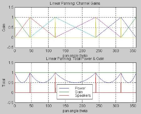
Fig. 3.4. Linear, constant gain panning for five channels: (top) channel gains, (bottom) total power and total gain.
Unfortunately, constant gain does not yield constant loudness. The average pressure variation D p in front of a loudspeaker is proportional to the total gain, the intensity level is proportional to the square of D p, and subjective loudness is proportional to intensity depending on the spectrum of the signal. Thus loudness is proportional to the total power and not the total gain. (See Appendix A for more details.) We see from the bottom of Figure 3.4 that the total power drops by half for an image panned directly between two speakers. This leads to a decrease in loudness that is often perceived as an increase in image distance. This primary fault of constant gain panning has led to its rare use in audio except under very low budget situations.
This desire for constant loudness for all panning angles led to constant power as a criterion for optimizing pan pots, as in Gerzon’s eighth criterion above. The first constant power pan pot was thought to have been designed by Garrity and Hawkins at Disney Hyperion studios for use with their Fantasound process [3]. Most pan pots in use today are based on pair-wise, constant power methods. We first describe a two-channel panning law and then proceed to a five-channel one.
The most elegant way of ensuring constant power is the use of the trigonometric identity in Eq. (3.5) [37].
(3.5)
Griesinger states that the cosine law also corresponds to the directional dependence of the Blumlein coincident array, which is formed by placing microphones with figure of eight responses at a 90º angle [2]. Other constant power panning laws have been considered in the literature, including [38] [39].
If the gain of one channel varies as the sine of q , and the gain of the other varies as the cosine of q , then their total power (the sum of the squares) is guaranteed to be constant. To allow for wide angles between the two speakers, q pan is first mapped to an angle q m between 0º and 90º. The gains for the right and left channels are determined as functions of q m, as shown in Eqs. (3.6) to (3.8).
(3.6)
(3.7)
(3.8)
These constant power gains for the two-channel case are plotted against q m in Figure 3.5. Here we note that the total system power is indeed constant, whereas the total gain increases to almost 1.5 times its value directly between the speakers.
With some additional conditional logic, two-channel constant power panning may be adapted to the multichannel case. Table 3.2 shows these channel gains for panning angles from 0º to 359º and arbitrary speaker angles.
Table 3.2. Constant power panning for five speaker channels
| Range of q pan | Channel gain gi (all angles in degrees) |
Figure 3.6 shows the channel gains, total gain, and total power for the five-channel, constant power panning law.
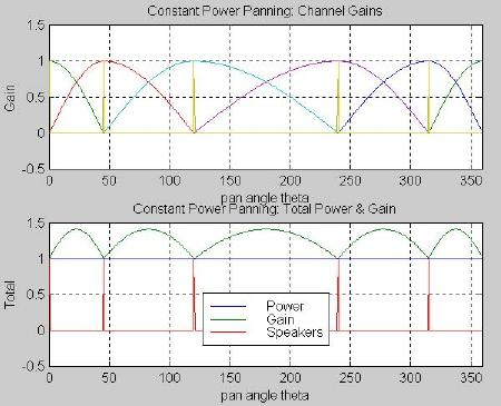
Fig. 3.6. Constant power panning for five channels: (top) channel gains, (bottom) total power and total gain.
Velocity and Energy Vector Optimization
Theory. Now we turn to more esoteric optimizations for pan pots. Throughout his long history with surround sound, Gerzon used the concepts of velocity vectors, energy vectors, and "phasiness" to optimize panning laws [29] [40] [31] [35] [11]. He emphasized that he did not consider these theories to be accurate models of acoustics or human localization. Instead, he found that algorithms optimized using these theories are the ones that best conform to his design criteria for surround sound systems and pan pots. (Phasiness, described in [40], [41], and [42], will not be considered here.)
The following description of these concepts is based on Gerzon’s work [29] [11]. Suppose that the i-th speaker in Figure 3.3 emits a sound "magnitude" mi whose physical nature we do not yet specify. The total sound "magnitude" for a central listener is the sum of the magnitudes from each loudspeaker.
Total magnitude (3.9)
The resulting vector direction can be found by drawing vectors from the center to each speaker of length mi and taking their vector sum in Cartesian form as in Eqs. (3.10) and (3.11).
Vector x-axis component (3.10)
Vector y-axis component (3.11)
This vector can then be normalized to a unit vector by dividing by the total magnitude sum from Eq. (3.9). This unit vector, shown in Eqs. (3.12) and (3.13), is described in polar form with length r (r ³ 0) and direction q . For single sound sources, q is the direction of the sound source and r = 1.
Unit vector x-axis component 
(3.12)
Unit vector y-axis component 
(3.13)
If the "magnitude" mi is the actual gain gi of a signal fed to the i-th speaker, then the sum in Eq. (3.9) is the total pressure gain and the unit vector above is called the velocity vector gain at the listener. In this case, we arrive at Eqs. (3.14) and (3.15).
Velocity vector magnitude r = rV = (3.14)
Velocity vector direction q = q V = 
(3.15)
Gerzon found that the velocity vector magnitude rV describes the degree of phantom image movement according to interaural phase location theories as the listener’s head is rotated. If rV < 1, the phantom image rotates in the same direction as the head (undesirable). If rV > 1, the phantom image rotates in the opposite direction (desirable).
Makita [43] found that the velocity vector direction q V is "the apparent sound localization direction according to low-frequency interaural phase localization theories (particularly apparent below around 700 Hz) when the listener faces the apparent sound source [29]." The velocity vector direction is often referred to as the Makita direction. Not described by this theory is the localization direction of a listener not facing the sound source.
If the "magnitude" mi is instead equal to the square of the gain gi, then the unit vector is called the energy vector. Its respective components are the energy vector magnitude rE and energy vector direction q E .
Energy vector magnitude r = rE = (3.16)
Energy vector direction q = q E = 
(3.17)
Gerzon found that the value of rE is a good predictor of the degree of image movement as a listener moves away from the central position [29]. This value can never exceed unity, and only equals unity when a sound is emitted by only one loudspeaker. The degree of angular movement of a phantom image, relative to loudspeaker azimuths, caused by a given degree of listener movement is proportional to 1- rE. Thus a value for rE of 0.95 corresponds to about one third the degree of image movement as a value of 0.85. (Moorer refers to the energy vector as the power vector [11]. He also states that if mi in Eq. (3.9) is made equal to gain gi to the 7/4 power, then the "power" vector corresponds to high frequency localization better than squaring gi [44]. However, no experimental evidence of this is referenced.)
The energy vector direction q E is "used to determine apparent sound direction for listeners facing the apparent sound source for frequencies between 700 Hz and 3.5 kHz, although it will be realized that these frequencies are ‘fuzzy’ and that there is in practice overlap in the frequency ranges at which q V and q E are used to determine localization [29]." Gerzon notes vaguely that rE is useful in this same frequency region and also below it for the phase-incoherent cases such as off-center listening.
Gerzon summarizes these ideas by saying that q V and q E should be equal for localization consistency in different frequency ranges (Gerzon’s criterion 1). He also states that rE should be as large (as near to unity) as possible, and as constant and smooth as possible. The value of rV should be reasonably close to unity, but this is less important than the constraints on rE.
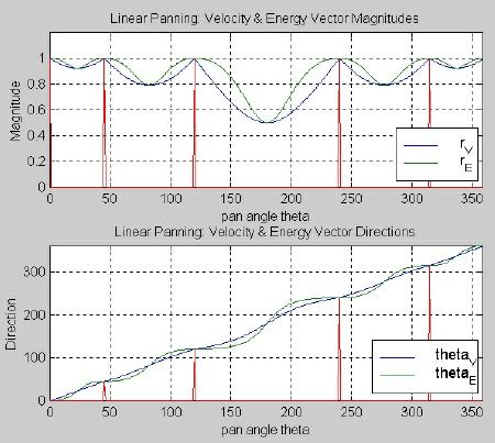
What do the velocity and energy vector components look like for the constant gain and constant power panning laws? Figure 3.7 shows these values for the two-channel versions of each panning law. The plots for each of the vector magnitudes are fairly similar, and neither rV nor rE is very close to unity. In both panning laws, q V corresponds very closely to the ideal localization scenario in which the perceived localization azimuth is the same as the desired panning angle (a y = x function). q E varies around q V, and it varies slightly less so for constant power panning.
(a) | (b) |
The vector directions, shown in the bottom of Figure 3.7 (a) and (b), predict that localizations for the low and high frequency ranges should correspond only for phantom images located at the speaker azimuths (± 45° ) or centered between them (0° ). Phantom images with high frequency components and at locations other than these should show a tendency to be localized closer to the nearest speaker (rather than the center). This tendency for an image to be pulled closer to a speaker location is called the "detent effect."
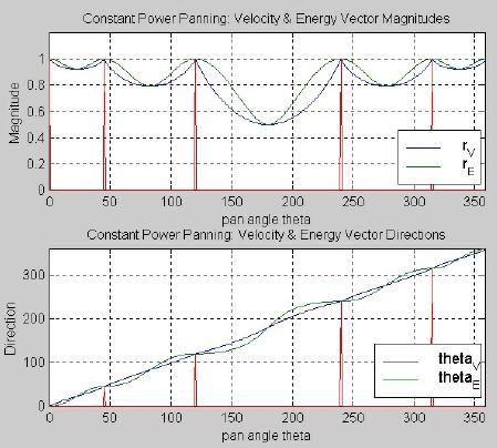
In Figures 3.8 and 3.9, we see the velocity and energy vector components for the five-channel versions of the constant gain and constant power algorithms. As before, the "spikes" in the plots denote speaker locations. Just as in Figure 3.7, the magnitudes are essentially the same for constant gain and constant power.
In both cases, the local minima of each magnitude are functions of the distance between adjacent speakers. (This may be a symptom of mapping q pan to q m before computing the vector components, something that Gerzon did not do.) The vector directions for both panning laws are also similar, as expected. We should expect less accurate localization with the constant gain case because its values for q V and q E vary slightly more around the ideal y = x line than those for constant power.
Three-channel implementation. Gerzon developed a new three-channel panning algorithm to meet these vector-based criteria since previous pan pots had failed to do so [29]. He did this after proving the impossibility of the velocity and energy vector directions equaling for the two-channel case. As in most surround setups with a center speaker, his algorithm was required to have the right and left speakers equidistant from the center speaker. Figure 3.10 shows the three-channel system used in his design.
Fig. 3.10. Three-channel system.
The syntax in Table 3.3 will be used to aid in the clarity of the derivation.
Table 3.3. Syntax for Gerzon’s optimal three-channel pan pot
| i-th Channel Number | Channel Gain gi | Loudspeaker angle q i |
1 | R = g1 | q 1 = -q 3 |
2 | C = g2 | q 2 = 0 |
3 | L = g3 | q 3 = q 3 |
Taking the tangents of q V and q E, we obtain:
(3.18)
(3.19)
If we are to satisfy
q V = q E (3.20)
then the right hand sides of Eqs. (3.18) and (3.19) must be equal. This implies one of two solutions. Either
L = R , (3.21)
which yields a useless center-only image, or
,
(3.22)
which is derived through removal of the common (L - R) and sinq 3 terms. By removing the common L2cosq 3 and R2cosq 3 terms, Eq. (3.22) can be simplified further as
(3.23)
We can find a different expression for C by rearranging Eq. (3.18):
(3.24)
Gerzon then expresses L and R with an "ad-hoc normalization" that later will be changed to one yielding (approximate) constant power gain. In this manner, L and R are expressed in terms of a variable e :
(3.25)
(3.26)
Substituting Eq. (3.25) and (3.26) into (3.23), we find
(3.27)
Similarly, if they are substituted into Eq. (3.24), we find
(3.28)
Substituting Eq. (3.28) into (3.27), we arrive at the following quadratic formula in e :
(3.29)
The solution to this quadratic is found as
,
(3.30)
where
(3.31)
Gerzon’s derivation becomes somewhat vague at this point. We need to solve for e in terms of tanq V, which is defined in terms of L and R, which are functions of e . He notes that "one chooses the sign [for ± ] for which rE is largest in order to ensure the most stable sound localisation [sic]; for q V = q E > 0, this choice is + and for q V = q E < 0, this choice is - [29]." He describes how to normalize each of the three gains for constant power as in Eq. (3.32).
(3.32)
Gerzon does not provide the remainder of the derivation for his optimal three-channel pan pot.
The engineer has two things in his or her favor to complete the derivation. First, Gerzon provides a plot of L, C, and R as functions of panning angle q pan (where q pan is a fraction k of q 3). These are, of course, the final pan pot functions that need to be found. Second, we can test potential solutions (potential L, C, and R curves) by plotting the velocity and energy vector directions to ensure equality between them for all angles. Fortunately, a solution was found experimentally that graphically matched Gerzon’s gain curves and came extremely close to satisfying the q V = q E criterion. While a gap in mathematical reasoning exists in finding this solution, and it is not known whether it is the "best" solution, it was the only one found that works. This experimentally derived solution is the first original contribution of this project.
We continue the derivation by expanding Eq. (3.30) and letting e a and e b be its positive and negative solutions, respectively.
(3.33)
(3.34)
Next, we disregard Eq. (3.31) and let A = 1.
(3.35)
(3.36)
The channel gains are found to be functions of e a or e b. First q pan is mapped to our q m by normalizing it to a maximum of ± p /6 (± 30° ). Then a shifted and scaled version of q m replaces q 3 in e a or e b above. (This step essentially removes the loudspeaker angles from the derivation.) Table 3.4 lists the final channel gains. Note that this solution may be protected by a patent or other manner of intellectual property protection by Gerzon.
Table 3.4. Channel gains for Gerzon’s optimal three-channel pan pot
| Range of q pan | Channel gain gi (all angles in degrees) |
Gerzon’s optimal channel gains are plotted versus q m in Figure 3.11. Clearly, this is not a pair-wise panning law because all three channels have non-zero gains for all panning angles. Interestingly, the L and R gains each go negative for a quarter of the arc of q m. Note that this algorithm closely approximates constant power behavior.
Figure 3.12 shows the velocity and energy vector components for Gerzon’s optimal pan pot. Here we see that q V and q E are very nearly equal, deviating only slightly near the left and right speaker locations. We also see that rV and rE are very near their optimal values of one. Even if this does not match Gerzon’s intended solution exactly, it must be reasonably close for the vectors to behave this well.
Fig. 3.12. Gerzon’s optimal panning for three channels: vector components.
Five-channel optimal / constant power hybrid implementation. A simple five-channel panning algorithm may be developed by combining the optimal three-channel panning algorithm with constant power behavior between all the other speakers. This hybrid method promises to have the optimal algorithm’s advantages in the front sound stage, where it matters the most. Constant power behavior around the rest of the listener has the advantage of easy development based on current constant power laws. Table 3.5 and Figure 3.13 show the channel gains for this hybrid panning algorithm. Figure 3.14 shows its vector components.
Table 3.5. Hybrid optimal/constant power panning for five channels
| Range of q pan | Channel gain gi (all angles in degrees) | |
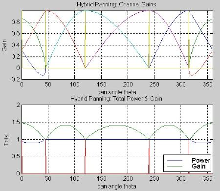
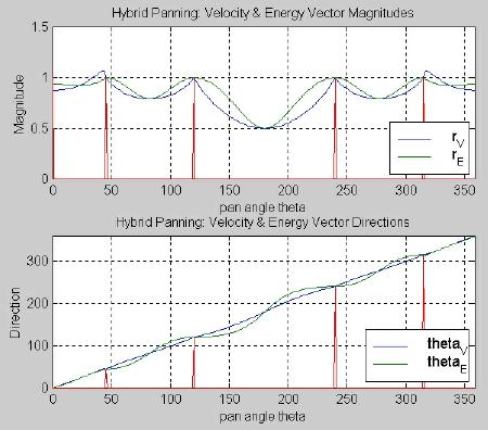
Fig. 3.14. Hybrid optimal/constant power panning for five channels: vector components.
Five-channel "optimal" implementation. With such a complex solution for the two-channel case, the reader may wonder how a five-channel "optimal" solution may be found. Gerzon considered the four-channel "optimal" case, and a five-channel solution is derived from this solution. The requirements for his four-channel system are that the speakers be equidistant from the center listening position, symmetric about the center line, and have equal angles between adjacent speakers. This last requirement is ignored for the derived five-channel version because such an arrangement would not conform to loudspeaker angles recommended elsewhere in the literature. (See Figure 4.5.) Despite this alteration, the derived algorithm approximated constant power behavior and had velocity and energy vector directions that were substantially equal.
Unlike the three-channel pan pot, which is essentially uniquely defined by q V = q E, Gerzon found that a four-channel panning law is not well constrained. After examining various trade-offs, he chose a "piecewise 3-speaker optimal" 4-speaker panning law as the best one. Consider his optimal three-channel panning law shown in the top of Figure 3.11. Imagine cutting off everything to the right of q m = 15° , where the right channel gain gi equals zero. (Note that the right channel gain is the one on the left that equals unity at q m = -30° .) Imagine further flipping the mirror image of everything from -30° £ q m £ 15° about the line at q m = 15° . One can visualize four individual speaker gains. As we shall see, this set of speaker gains has a smooth and reasonably constant value of rE over about 80% of its range.
A five-channel "optimal" panning algorithm can be found by combining the three- and four-channel algorithms in piecewise fashion. Let the speakers in the three-channel law be the right, center, and left speakers as usual. Then let the speakers in the four-channel law be the left, surround left, surround right, and right speakers. Figure 3.15 shows the gains for the resulting five-channel "optimal" algorithm. Combining the three- and four-channel laws into a one suitable for today’s five-channel systems was the second original contribution of this project.
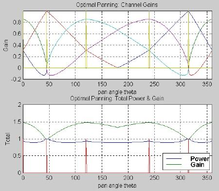
Fig. 3.15. Optimal panning for five channels: (top) channel gains, (bottom) total power and total gain.
Depending on the panning angle, this panning law has various numbers of channels with non-zero gains. When q pan = q 1 or q pan = q 3 , the right and left speaker azimuths respectively, only one speaker channel is active -- namely the right or left channel. When q pan = 180 ° , the line of symmetry in the four-channel optimal law, only the surround left and surround right channels are active. For all other panning angles, three speaker channels have non-zero gains.
The gains for the five-channel optimal algorithm are described in Table 3.6.
Table 3.6. "Optimal" panning for five channels
| Range of q pan | Channel gain gi (all angles in degrees) |
If Else | |
The vector components for the five-channel optimal algorithm are shown in Figure 3.16. We note the similar shape of the magnitude curves for the inner four-channel region with the outer three-channel region. We again notice that the dip in the magnitudes is to the rear of the listener, where the speakers are the greatest distance from each other. Looking at the vector directions, we see that they differ from each other only slightly all the way around the listener. They differ the most at the edges of the four-channel optimal algorithm: just to the right of the right speaker (at 45° ) and just to the left of the left speaker (at 320 ° ). According to Gerzon’s theories, localizations of low and high frequencies should differ the most in these regions.
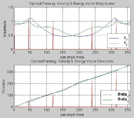
Fig. 3.16. Optimal panning for five channels: vector components.
Azimuthal Harmonic Optimization
We now examine one last method of optimization, one that relies on azimuthal harmonic theory. While Moorer introduced this subject to the author [11], this theory was developed originally by Cooper and Shiga [45] and expanded to three dimensions by Gerzon [46]. Our description of azimuthal harmonic theory, almost entirely based on Moorer [11], is the horizontal-only case of the more general spatial (or "spin") harmonic theory. Note that the Ambisonic surround sound format of Gerzon is based on both spatial harmonic theory and the velocity/energy vector theory already mentioned.
Assume for a moment that humans are only sensitive to sound waves arriving from the horizontal plane. Consider the head centered on a point, and let f(q ) represent the sound pressure wave incident on that point from any azimuth q . Since q is an angle on a circle, f(q ) is periodic in q . We therefore can represent f(q ) as a Fourier series:
(3.37)
If f(q ) is known, we can determine the coefficients an and bn as follows:
(3.38)
(3.39)
We are interested in a function describing a single sound source appearing at an angle f . Eq. (3.40) shows this function in terms of the Dirac delta function d (q ).
(3.40)
This function results in the following coefficients.
(3.41)
(3.42)
If we substitute these coefficients into Eq. (3.37) and simplify using the cosine sum of angles formula, we find the horizontal harmonic expansion of our directivity function to be:
,
(3.43)
where q is any azimuth, f is the azimuth of the incident sound wave, and n is the azimuthal harmonic number (in units of 1/degrees azimuth).
Now we consider the situation of a horizontal-only surround sound system with N loudspeakers. For signals fed to the i-th speaker with gain gi, the contribution of the i-th speaker to directivity is:
(3.44)
The sampled, total directivity function then may be represented as the sum of the individual speaker contributions:
(3.45)
The goal of the surround sound system is to reproduce as closely as possible the original directivity function f(q ) with fs(q ) . The task then is to calculate the unknown channel gains by fitting the directivity function in Eq. (3.43) to the directivity function from our unique speaker set-up in Eq. (3.45). This may be done using a least-squares approximation:
(3.46)
We arrive at the following set of N linear equations for the N unknown gains after some manipulation:
,
(3.47)
where k = 1, 2, …, N.
Cooper and Shiga’s azimuthal sampling theory [45] states that with N speakers spaced equi-angularly, we cannot recreate more than floor (N/2) azimuthal harmonics without azimuthal aliasing. (It is unclear how azimuthal aliasing manifests itself perceptually.) Since N = 5 in our case, we cannot recreate more than the first two terms (n = 1, n = 2) if we had equi-angularly spaced speakers. (In this case, the bound on the cosine summations in Eq. (3.47) would be 2.) Moorer describes the dilemma for our situation:
Since our speakers are not equi-angular it is spatial sampling with unequal steps. The most conservative reading of the sampling theorem dictates that the highest spatial harmonic is then related to the largest step [between adjacent speakers]. This limits us for practicality to the first term only. In fact, if any of the angles between successive speakers is greater than 90 degrees, then even the first spatial harmonic can not be recreated [without spatial aliasing?] ... It says that we cannot hope to achieve a high degree of directionality, even with 5 speakers, since we can only recreate the zero-th and first spatial harmonics [11].
Setting aside the question of azimuthal aliasing, the calculation of the speaker gains continues. When we have N > 3 speakers and use only the zero-th and first spatial harmonics, we have only three free parameters. Thus Eq. (3.47) is a rank three underdetermined system of equations. To obtain a solution to Eq. (3.47), we must apply two more linearly independent equations as constraints. Moorer told to the author that a perfectly acceptable solution could be found by forcing the 2nd order spatial harmonics to zero [47]. These two constraints, shown in Eqs. (3.48) and (3.49), raise the rank of the system to five and enable us to solve for each of the channel gains. Note that this is one pair of many possible constraints that could used to solve the system of equations.
(3.48)
(3.49)
The channel gains found using this set of constraints are plotted in Figure 3.17. Here we see that all channels are active for any given panning angle. Like Gerzon's optimal algorithm, the channel gains do go negative over certain panning ranges. We also note that the total gain is constant and the total system power increases substantially between the surround left and surround right speakers.
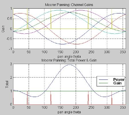
Fig. 3.17. Moorer azimuthal harmonic optimized panning for five channels: (top) channel gains, (bottom) total power and total gain.
In Figure 3.18, we see very odd behavior for the Moorer algorithm’s vector components. Both the magnitudes and the directions had to be processed with unwrapping algorithms, and the spikes in rV are spurious results of that unwrapping. The energy magnitude rE seems rather low compared to previous values. While q V looks very good, q E does not match it except in the range below about 90 degrees.
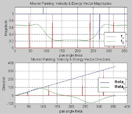
Fig. 3.18. Moorer azimuthal harmonic optimized panning for five channels: vector components.
The azimuthal spectra for all panning algorithms are shown in Figure 3.19. For each panning law, the sampled directivity functions were computed using Eq. (4.45) and plotted in the azimuthal frequency domain up to the second harmonic. The Moorer algorithm has the lowest second harmonic amplitude of all algorithms -- down approximately 6 dB from linear, constant gain panning. Our chosen constraint on the Moorer panning matrix yielded a relatively low but nonzero second harmonic. The other algorithms show higher second harmonics, presumably because of the addition of aliasing artifacts. The zero-th and first spatial harmonics for the Moorer algorithm are almost identical in magnitude. In all other algorithms, the first harmonic is down at least 0.5 dB from the zero-th harmonic. Recall that it is unclear how (or if) differences between the algorithms’ azimuthal spectra will be audible.
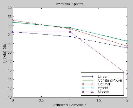
Fig. 3.19. Azimuthal spectra for all panning algorithms.
A few of the theories on which these panning laws are based have undergone some peer review. Gerzon determined that laws based on velocity and energy vector theory were superior to all pair-wise panning methods [29]. However, Mertens [48] [49] criticized the Makita velocity vector theory because (1) the stereophonic wavefront "cannot be identified with that of a single source within even a rather small region of space," and (2), Makita’s calculations did not agree with his experimental results [36]. Moorer stated that panning laws with three or more non-zero gains, as in his spatial harmonic based algorithm, would have a wider "sweet spot" than pair-wise methods such as constant power panning [11].
Willcocks and Badger give a good overview of the subject [36]. They offer the following comparison between pair-wise panning laws (i.e., constant power) with spherical harmonic methods. Recall that the spatial harmonics described with the Moorer algorithm are the two-dimensional version of the more general, three-dimensional spherical harmonics. (They refer below to pair-wise panning as pair-wise mixing or PWM.)
If a PWM system is used, image stability will be worse than for a spherical harmonic based system only at the exact center of a precisely set up speaker array, fed with the correct signals. Off center, beyond the point at which the additional crosstalk begins to introduce phasiness problems (a function of frequency), the localization for a discrete PWM system will always be better than for a system with crosstalk, whatever the polarity of crosstalk. Of course, localization of phantoms will not be correct [with PWM], but will always lie between or at the energized speaker locations, from any location inside or outside the array [36].
While Willcocks et al. do not compare the size of the sweet spots of these two systems, they state that the behavior of a PWM system will be superior outside the sweet spot. For the curious, Fels et al. [50] have developed a method for increasing the size of the sweet spot or "listening zone" for pair-wise mixed material.
Table 3.7 summarizes how or if the panning algorithms meet the pan pot criteria from the beginning of the chapter.
Table 3.7. Analytical comparison of panning algorithms using Gerzon's criteria
(Previous Chapter) <- Main Page -> (Next Chapter)
Jim West, University of Miami, Copyright 1998